tl;dr
- many analyses in the social sciences require many R packages
jmvmakes these common analyses available from one R packagejmvcan be used from jamovi, a graphical statistical spreadsheet, making it super-accessible
introducing jmv
There are many tremendously useful R packages for the social sciences (and similar fields), such as car, afex vcd, etc. Although running basic analyses (such as t-tests or ANOVA) with these packages is very straight forward, it is typically necessary to perform a number of supplementary analyses to accompany them; post-hoc tests, effect-size calculations, bias-corrections, and assumption checks. These additional tests often require the use of many additional R packages, and can make reasonably standard analyses quite time-consuming to perform. For example, in the book Discovering Statistics Using R by Andy Field (a popular textbook in the social sciences), the chapter on ANOVA alone recommends the use of 7 packages.
jmv simplifies this whole process by bringing all of these packages together and makes doing the following analyses with their most common supplementary tests, corrections and assumption checks as easy as possible:
- Descriptive statistics
- T-Tests
- ANOVA
- ANCOVA
- Repeated Measures ANOVA
- Non-parametric ANOVAs
- Correlation
- Linear Regression
- Contingency Tables
- Proportion Tests
- Factor Analysis
and coming soon:
- Logistic Regression
- Log-linear Regression
jmv aims to make all common statistical tests taught at an undergraduate level available from a single package.
An ANOVA
Let’s begin with a simple, familiar analysis – an ANOVA. In this example we use the ToothGrowth dataset from R, and explore whether different food supplements and their dosage affect how much a guinea pig’s teeth grow. We’ll specify len to be the dependent variable, and supp and dose to be the factors.
library('jmv')

data('ToothGrowth')

jmv::anova(ToothGrowth,
           dep = 'len',
           factors = c('supp', 'dose'))
##
##  ANOVA
##
##  ANOVA
##  ───────────────────────────────────────────────────────────────────────
##                 Sum of Squares    df    Mean Square    F        p
##  ───────────────────────────────────────────────────────────────────────
##    supp                    205     1          205.4    15.57    < .001
##    dose                   2426     2         1213.2    92.00    < .001
##    supp:dose               108     2           54.2     4.11     0.022
##    Residuals               712    54           13.2
##  ───────────────────────────────────────────────────────────────────────
This produces what should be a familiar ANOVA table. You have likely seen something like this in R before, though perhaps not as nicely formatted.
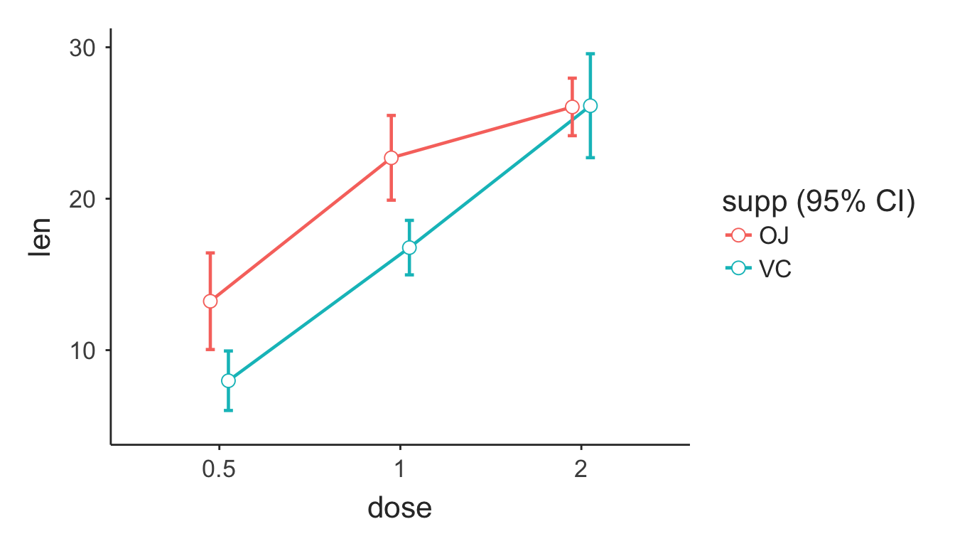
Where jmv really comes into its own, is with additional options. In the following example we will perform the same analysis, but additionally requesting effect-size, post-hoc tests, homogeneity of variances tests, descriptive statistics, and a descriptives plot:
library('jmv')

data('ToothGrowth')

jmv::anova(ToothGrowth,
           dep = 'len',
           factors = c('supp', 'dose'),
           effectSize = 'eta',
           postHoc = c('supp', 'dose'),
           plotHAxis = 'dose',
           plotSepLines = 'supp',
           descStats = TRUE,
           homo = TRUE)
##
##  ANOVA
##
##  ANOVA
##  ────────────────────────────────────────────────────────────────────────────────
##                 Sum of Squares    df    Mean Square    F        p         η²
##  ────────────────────────────────────────────────────────────────────────────────
##    supp                    205     1          205.4    15.57    < .001    0.059
##    dose                   2426     2         1213.2    92.00    < .001    0.703
##    supp:dose               108     2           54.2     4.11     0.022    0.031
##    Residuals               712    54           13.2
##  ────────────────────────────────────────────────────────────────────────────────
##
##
##  ASSUMPTION CHECKS
##
##  Test for Homogeneity of Variances (Levene's)
##  ────────────────────────────────────────────
##    F       df1    df2    p
##  ────────────────────────────────────────────
##    1.94      5     54    0.103
##  ────────────────────────────────────────────
##
##
##  POST HOC TESTS
##
##  Post Hoc Comparisons - supp
##  ────────────────────────────────────────────────────────────────────────────
##    supp         supp    Mean Difference    SE       df      t       p-tukey
##  ────────────────────────────────────────────────────────────────────────────
##    OJ      -    VC                 3.70    0.938    54.0    3.95    < .001
##  ────────────────────────────────────────────────────────────────────────────
##
##
##  Post Hoc Comparisons - dose
##  ─────────────────────────────────────────────────────────────────────────────
##    dose         dose    Mean Difference    SE      df      t         p-tukey
##  ─────────────────────────────────────────────────────────────────────────────
##    0.5     -    1                 -9.13    1.15    54.0     -7.95    < .001
##            -    2                -15.50    1.15    54.0    -13.49    < .001
##    1       -    2                 -6.37    1.15    54.0     -5.54    < .001
##  ─────────────────────────────────────────────────────────────────────────────
##
##
##  Descriptives
##  ───────────────────────────────────────
##    supp    dose    N     Mean     SD
##  ───────────────────────────────────────
##      OJ     0.5    10    13.23    4.46
##      OJ       1    10    22.70    3.91
##      OJ       2    10    26.06    2.66
##      VC     0.5    10     7.98    2.75
##      VC       1    10    16.77    2.52
##      VC       2    10    26.14    4.80
##  ───────────────────────────────────────

As can be seen, jmv can provide many additional tests and statistics relevant to the main tests, but with far less effort.
You can explore additional options for the jmv ANOVA here, and the other tests and their available options here.
jamovi integration
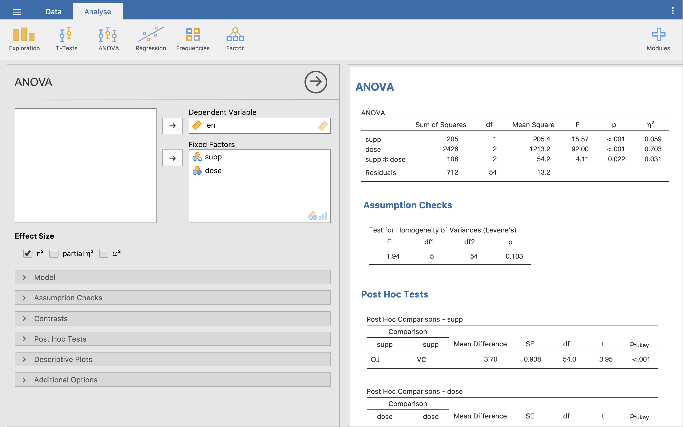
jmv is also useable from the jamovi statistical spreadsheet. jamovi makes a range of analyses accessible to a broader audience by making them available from a familiar, spreadsheet user-interface. jamovi can also make the underlying R code for each analysis available, making it easy for people to learn R, and transition to R scripting if they like.
Here is exactly the same analysis as above, having been performed in jamovi.

summing up
jmvmakes a whole suite of common analyses from the social sciences very easy to performjamovimakes these even easier to perform
jmv is available from CRAN
jamovi is available from www.jamovi.org
Comments