tl;dr
Ever wanted to try doing an evidential analysis? You may have found it difficult to find a statistical platform to do it. Now there is the jamovi module jeva which can provide log likelihood ratios for a range of common statistical tests.
Update - 20 Feb 2024
Version 0.1.0 and later now features two-way factorial ANOVA, repeated measures ANOVA and diagnostic testing for a 2 x 2 table.
The factorial ANOVA allows two fixed factors, while the repeated measures analysis allows one-way and mixed between-participants variable (only one allowed). Where possible p values are also displayed to allow comparison with conventional frequentist analyses.
Both ANOVAs do model comparisons for main effects and interactions. In addition, it is possible to enter 2 contrasts. The strength of evidence for each of these is given, including the evidence for the first contrast versus the second. The comparison between contrasts illustrates the power of the evidential approach using log likelihood ratios, since a p value cannot be calculated here.
Options for correction for parameters have been added to analyses. For these ANOVAs there are 4 options: None, Occam’s Bonus (default), AIC and AICs.
The diagnostic test analysis produces the usual statistics including likelihood ratio, PPV, NPV and Youden’s Index J. Null values for the sensitivity and specificity can be set to compare with those obtained by the data. Likelihood function plots of sensitivity and specificity can also be done. Finally a Fagan nomogram is available which graphically links prior probability (prevalence) to posterior probability.
… and there are now loadable data sets available from the jamovi Data Library (see Open file menu).
Acknowledgements: Most of the analyses have used templates provided by the main set of jamovi analyses, produced by the jamovi team. So, I am extremely grateful to the amazing jamovi team in allowing me to appropriate their analyses in this way. I am particularly grateful to Jonathon Love who has provided me with extraordinary support and advice. Thank you!
Original Post
Imagine for a moment that we wish to carry out a statistical test on our sample of data. We do not want to know whether the procedure we routinely use gives us the correct answer with a specified error rate (such as the Type I error) – the frequentist approach. Nor do we want to concern ourselves with possible a priori probabilities of hypotheses being true – the Bayesian approach. We need to know whether a statistic from this particular set of data is consistent with one or more hypothetical values. Also, let’s say that we weren’t happy with how much data we had collected (a familiar problem?), and just added more when convenient. Welcome to the likelihood (or evidential) approach!
In my view, using just LLRs is actually the simplest and most direct procedure for making statistical inferences. I will not here rally arguments in support of the likelihood approach, but merely point the reader to better sources: (Edwards 1992, Royall 1997, Dennis, Ponciano et al. 2019)
For the given data, the likelihood approach calculates the natural logarithm of the likelihood ratio for two models being compared. So, it should be possible to do likelihood analyses in any of the major statistical packages, right? Well, it is possible to obtain log likelihood and deviance in any procedure that uses maximum likelihood. So yes, in SPSS when you run a logistic regression you will find -2 Log likelihood in the Model Summary. The same statistic is given by SAS in the Model Fit Statistics. In Minitab the statistic is labelled deviance. Finally, Stata gives the log likelihood. (I am grateful to Professor Sander Greenland for pointing out the availability of these statistics in common statistical packages.) In R, deviance statistics are given using glm, and logLik can be used to extract the log likelihood. In jamovi, the deviance and AIC are available, for example in binomial logistic regression. Although log likelihoods are available, we need to know which ones to use and how to calculate a log likelihood ratio.
Calculating the LLR
Bear with me, or skip this section if you have never coded.
Now, I want to calculate the LLR for some data that consists of measurement data in 2 independent groups. I want to know how much more likely is the model with fitted means compared to the null model (one grand mean only). I will assume equal variances in the 2 groups. OK, this is just an independent samples t test. Working in R, we first create the data (representing increased hours of sleep following a drug):
mysample <- c(0.7, -1.6, -0.2, -1.2, -0.1, 3.4, 3.7, 0.8, 0.0, 2.0)
treat <- rep(1:0,each=5)
We then do separate analyses for the means model (m1) and the null model (m2):
m1=glm(mysample~treat)
m2=glm(mysample~1)
The easiest way to get the log likelihoods is using the logLik function (note the capital L in the middle). Remembering that the log of a ratio is the same as subtracting the log of the denominator from the numerator:
logLik(m1) - logLik(m2)
This prints:
'log Lik.' 3.724533 (df=3)
This is the answer we are looking for, and represents strong evidence against the null hypothesis, see Table 1 below. The output also tells us that the fitted model (m1) has 3 parameters, which are: the variance and the two group means. The null model only has the variance and the grand mean.
There is a widely held misconception that deviance for a normal model is −2 x log likelihood (−2LL), e.g. Goodman 1989. It is not, it is only the sums of squares (SS). Only for non-normal models (such as Poisson and binomial) does the deviance equal −2LL. However, the unexplained SS (deviance in normal data) can provide likelihoods (see Glover and Dixon 2004 for details). We can use the following formula using the residual SS (RSS) and total SS (TSS) to calculate the LLR for a fitted model versus the null:
Where N is the total sample size. In R we do this either using the SS given in an ANOVA table or from the deviances. We will use the latter:
-length(m1$y)/2*(log(m1$deviance) - log(m2$deviance))
This gives us the same result as earlier. Another way to do the analysis is to use Akaike Information Criterion AIC, which uses log likelihoods but takes into account the number of parameters in the two models:
(m2$aic - m1$aic)/2
This gives us 2.724533, exactly 1 less than the previous answer. The reason for this is that the LLR is penalized for increasing the complexity of the model by 1 parameter (for the two group means) over the null model. Some recommend this or a similar penalty depending on the sample size (Glover 2018), although if we compare the p value produced by the corrected likelihood ratio test with that produced by the regular t test, then such correction seems harsh.
I tried asking ChatGPT: “how to calculate a log likelihood ratio for independent samples t test using R?”. The answer was fine, calculating null and means models, but gives in the final line:
LLR <- 2 * (logLik(model1) - logLik(model0))
The use of logLik function is good, but of course, the 2 times multiplier is wrong . This is, I think, an attempt to relate it to the deviance. As we noted earlier, it is only identified with −2LLR in certain circumstances.
I think the reader gets the idea. There are issues about using the right functions appropriately and the number of parameters to consider. Doing a likelihood analysis of a simple independent samples t test is not so straightforward. If we wanted to use Welch’s test on the data, or wanted to compare a model with a null hypothesis value different from 0, it would be even more difficult to calculate the LLR. It would require quite a few more lines of code.
Using jeva
When I published my book a few years ago (Cahusac 2020) I was surprised how difficult it was to find software that would calculate LLRs for common statistical tests. This led me to produce a package in R called likelihoodR (Cahusac 2022). Since then, I discovered that the best platform was jamovi, where users can produce modules for custom analyses. So I produced a module called jeva (jamovi evidential analyses). Each analysis has an option to give explanatory text, to help explain what the findings of a particular analysis means in terms of the evidential framework used.
Independent Samples t test
The jeva analysis of 2 independent samples t test is given in Figure 1. This is for the same data given earlier (increased hours of sleep in males and females following a drug).
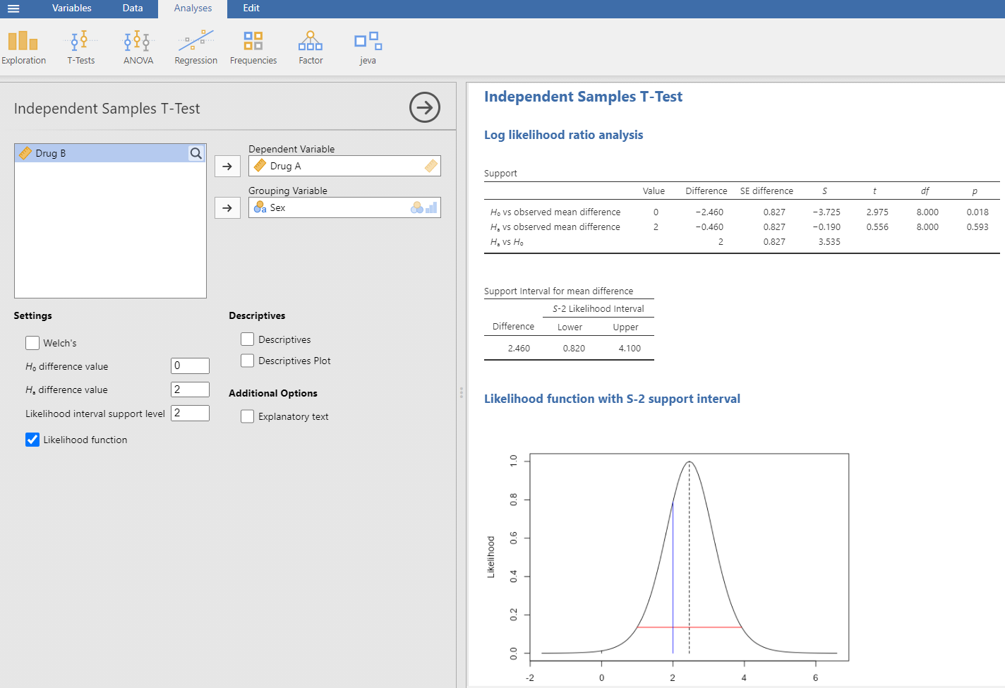
Figure 1: jeva analysis of 2 independent samples. The dialog box is on the left, where we select the data and options appropriate for our analysis. The output is on the right.
The analysis shown assumes equal variances, otherwise we could select Welch’s. In the Support table, the LLR (S) for vs observed mean difference is −3.725. Why negative? Well, it depends on what order we specify the two models, and we have specified the first. This means that the null hypothesis is much less likely than the observed mean difference. To see how much less likely, we use , or the inverse, 41.5 times less likely. In the dialog box I have entered 2 for , which was suggested as a clinically important sleeping time for the effect of the drug. The Support table gives the LLR for this value versus the observed difference in means as (1.2 times different), which represents a trivial difference. The 3rd row in the table gives the LLR for vs as 3.535, representing strong evidence ( is 34.3 times more likely than the null). This is a comparison which can easily be done using the likelihood approach – no p is available. The likelihood function at the bottom shows the positions of the different hypothesis values and the observed mean difference (2.46, vertical dashed line). The horizontal red line is the likelihood interval for S-2 (values given in the Support interval for mean difference box above it), closely corresponding to the 95% confidence interval. The vertical black line is at 0, and the vertical blue line is at 2. With familiarity, it is easier to think in terms of the LLRs, known as support values S, rather than the exponentiated values. A useful comparison table is given in the Additional Option of Explanatory text, and is reproduced in Table 1 below (based on a table given by Goodman (1989)).
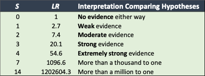
Table 1: Interpreting the support S obtained in an LLR analysis for one hypothesis value versus a second. The middle column shows the likelihood ratio, which is . The right column gives the interpretation. Negative S values just mean that the second hypothesis value is more likely than the first.
The natural log is used in all the calculations and the LLRs can simply be added together, for example when accumulating the evidence of the same phenomenon. Do you want to add to your study data? That’s not allowed using the frequentist paradigm, but fine in the likelihood approach. It also makes meta-analysis easy, just add the S values together.
Odds Ratio
Let’s look at another analysis in jeva, the odds ratio (OR). These data are from a double-blind randomized clinical trial of folic acid supplements in pregnant women. About half received folic acid and half received placebo during pregnancy. The outcome was whether the babies born had a neural tube defect or not. Putting the data into jamovi, the first part of the output gives us the summary 2 x 2 table:

Since the intervention (folic acid) appeared to reduce the defect, the OR was less than 1. In fact, it was 0.283. A more complete picture of the analysis is shown in Figure 2.
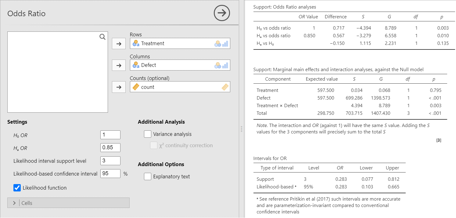
Figure 2: Doing an odds ratio analysis in jeva. On the left is the dialog box giving settings and options. On the right is the output.
The settings in the dialog box show that the null hypothesis is 1, as it normally should be, but we can specify another value if necessary. We can also select an alternative hypothesis value and here we have entered 0.85. This could be a value suggested as the minimal clinical effectiveness for the intervention.
The first line of the Support: Odds Ratio analyses table gives us the strength of evidence for the null versus the observed OR as S = −4.39. This means that there is extremely strong evidence that the observed OR differs from the null value of 1. (The trial was discontinued and all women were given folic acid). We will from now on refrain from exponentiating it to obtain how many times more likely, and use the S values alone. The next line in the table gives the strength of evidence for the alternative hypothesis of 0.85 compared with the observed OR. At −3.28 the evidence is strong that the observed value differs from the minimal clinical effectiveness value, i.e. the observed OR is much better than the required minimum. The final line in the table pits the alternative hypothesis value against the null. With S = 1.12, this suggests that there is at best weak evidence for a difference between these two values. In other words, although the observed OR strongly differs from the null and the alternative, the evidence suggests that these two values cannot be easily distinguished. For a comparison with the frequentist approach, the final column in the Support table gives the corresponding p values. These are consistent with the S value analysis (.003, .010 and .135 respectively). They are available through the likelihood ratio (or G) test, which means simply multiplying the S values by 2 and using the distribution to obtain the p values. Despite its name, the likelihood ratio test is not part of the evidential approach as it uses p values.
The next Support table (for marginal effects and interaction analyses) allows us to see if there are obvious differences in the marginal totals. Since similar numbers were allocated to folic acid and placebo, it is not surprising that S is close to 0. Analysis of the other marginal totals for presence of defect gives an extremely high S of 699, trivially telling us that most babies did not suffer from the defect. The 3rd row here repeats the S value from the first line of the previous table except that it is now positive. We are looking at the evidence for an interaction against the null model of no interaction. If we change the OR to something other than 1 then the values given in the first Support table would change, but not those in this table. The final line in this table calculates the S value, assuming that the 4 cells contain 1195/4 = 298.75. It is satisfying (to me at least) that the 3 previous components sum precisely to the total S = 703.715.
The table below the Support tables gives intervals for the observed OR. The first line gives the support interval. We have specified the level to be 3 in the dialog box. The lower and upper limits for the S-3 support interval are given, and correspond graphically to what is shown in the likelihood function curve below (see Figure 3). The next line gives a 95% likelihood-based confidence interval. It is close to the regular 95% confidence interval which jamovi gives as: 0.113 to 0.706. The advantage of the likelihood-based 95% confidence interval is that it is more accurate and is parameterization-invariant (Pritikin, Rappaport et al. 2017). The S-2 support interval is fairly close to both of these intervals: 0.101 to 0.676.
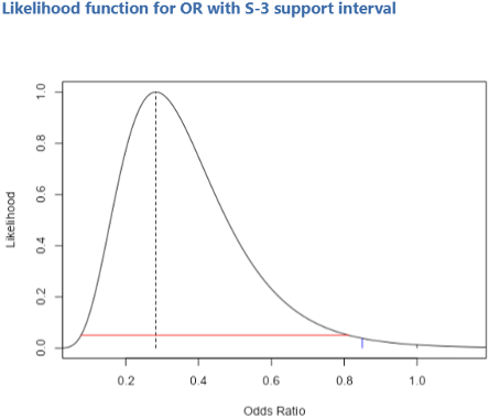
Figure 3: The likelihood function for the OR. The obtained value is shown by the dashed vertical line. The OR of 1 is shown as a vertical black line at the right side of the plot, and the OR of 0.85 is shown as the vertical blue line. The horizontal red line is the support S-3 interval. Both the and values lie outside the interval, since their S values versus the obtained OR exceed the absolute value of 3 (−4.39 and −3.28 respectively).
The LLR Support Interval
This identifies a supported range of values which are consistent with the observed statistic. In jeva it is denoted as S-X, where X can be any number between 1 and 100. The S-2 interval is commonly used since, as mentioned, it is numerically close to the 95% confidence interval. For the S-2 interval, it means that the values within the interval have likelihood ratios in the range 0.135 to 7.38, corresponding to e⁻² to e². Simply put, within an S-2 interval, no likelihoods are more than 7.38 times different from each other. Similarly, for the S-3 interval, likelihood ratios will range from 0.050 to 20.09, corresponding to e⁻³ to e³, and no likelihoods will be more than 20.09 times different from each other.
Variance Analysis
The categorical analyses all feature a variance analysis. When selected in the OR analysis we get this output:
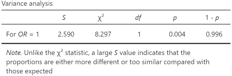
This analysis specifically addresses the issue of whether the variance of the counts in the cells vary more or less than we would expect by chance, assuming an OR of 1. With this particular analysis, we get S = 2.6 which is more than moderate evidence that the variance is different than expected. This broadly agrees with the value given earlier of S = 4.4 in the first Support table, although it is concerned with variance rather than the means (i.e. the expected frequencies). If the first count in the contingency table is changed from a 6 to 21, the obtained OR becomes very close to 1, and the Support table gives S = −0.001, indicating no difference from an OR of 1. However, the variance analysis now gives S = 2.9, almost strong evidence that the obtained OR is closer to 1 than we would expect (i.e. the variance is smaller than expected). The corresponding was very small at 0.001, with 1 – p = 0.026 (statistically significant). It is now answering the question as to whether the data fit the model too well – are the data too good to be true? This can be used to test whether data, like Mendel’s data (Edwards 1986), fit a model too well. Edwards (Edwards 1992), see especially pages 188-194, argued that the test could only be legitimately used for this purpose, and not what the test is normally used for (as a test of the means, i.e. the expected frequencies obtained from the marginal totals in an association test).
Finally
Currently, the jeva module has 10 common analyses: t tests, one-way ANOVA, polynomial regression, correlation, and 4 categorical analyses including McNemar’s paired test. In future, I aim to add factorial ANOVA, repeated measures ANOVA, logistic regression, and a sample size calculator for t tests (Cahusac and Mansour 2022).
Please do try out all the analyses. See how they compare with the other approaches. Where possible, p values are given to help compare with the conventional frequentist approach. I would be keen to hear any feedback, and you’ll get a £10 Amazon voucher (or regional equivalent) if you spot any errors!
Comments