tl;dr
- GAMLj is a jamovi module for general linear models, linear mixed-effects models, and generalized linear models
- GAMLj makes these classes of models accessible to a much broader audience
- Linear mixed-effects models make a great alternative to repeated measures ANOVA
One of the goals of jamovi is to make more sophisticated analyses accessible to a broader audience. A great example of this is the GAMLj module introduced here. If you’ve never used these models before, hopefully today I can convince you that with GAMLj they are within your reach, and that there are advantages to using these instead of more traditional analyses, such as repeated measures ANOVA.
For more technical readers, here is a feature list:
- OLS Regression (GLM)
- OLS ANOVA (GLM)
- OLS ANCOVA (GLM)
- Random coefficients regression (Mixed)
- Random coefficients ANOVA-ANCOVA (Mixed)
- Logistic regression (GZLM)
- Logistic ANOVA-like model (GZLM)
- Probit regression (GZLM)
- Probit ANOVA-like model (GZLM)
- Multinomial regression (GZLM)
- Multinomial ANOVA-like model (GZLM)
- Poisson regression (GZLM)
- Poisson ANOVA-like model (GZLM)
- Overdispersed Poisson regression (GZLM)
- Overdispersed Poisson ANOVA-like model (GZLM)
- Negative binomial regression (GZLM)
- Negative binomial ANOVA-like model (GZLM)
- Continuous and categorical independent variables
- Omnibus tests and parameter estimates
- Confidence intervals
- Simple slopes analysis
- Simple effects
- Post-hoc tests
- Plots for up to three-way interactions for both categorical and continuous independent variables.
- Automatic selection of best estimation methods and degrees of freedom selection
- Type III estimation
If that feature-list seems a bit overwhelming, it might be easier to think “GAMLj does a lot of stuff”. But don’t be put-off, GAMLj is suitable for beginners and advanced users alike.
Repeated Measures ANOVA
So the repeated measures ANOVA is something of a staple of the social sciences; it’s one of the most used tests. Unfortunately, it has the drawback that it cannot handle missing values – if any of the subjects in your data set have missing values they are excluded completely. It’s like they never participated in your study. This can be a real problem with the smallish sample sizes common in the social sciences. Fortunately, linear mixed models provide a simple alternative to repeated measures ANOVA, which is able to make use of these participants’ data. That means more power, less time spent collecting data, and better use of tax-payer’s money. What’s not to love about LME’s?!
So let’s begin with the Bugs data set provided with jamovi. Actually… the bad news is that the Bugs data set in jamovi is in wide-format. It looks like this:
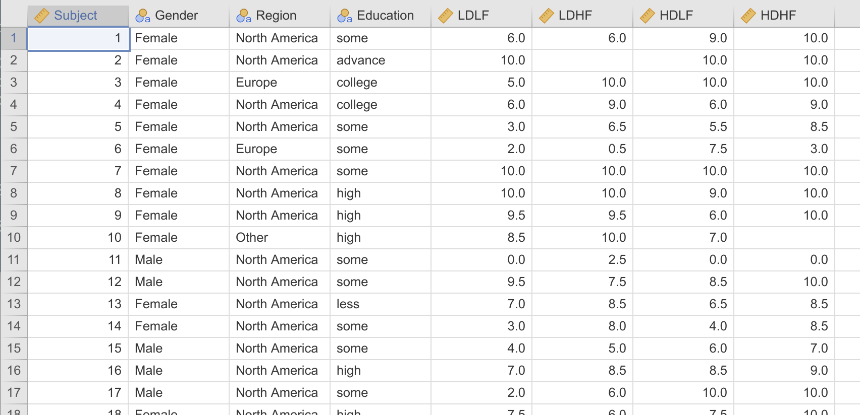
GAMLj requires the data be in long format. It needs to look like this:
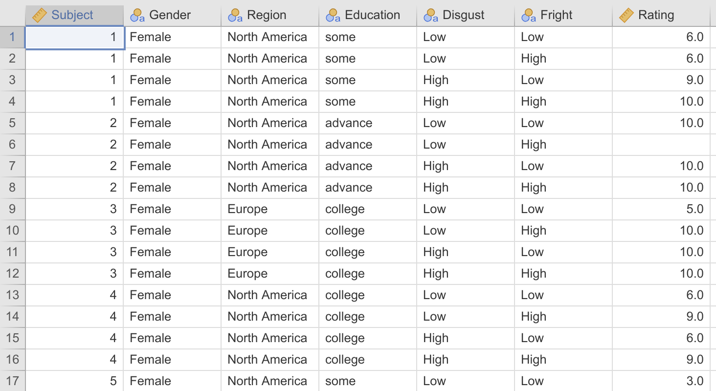
As you can see, in wide-format, each subject is represented as a row, with a column for each measurement of the dependent variable. In long-format, each measurement of the dependent variable is represented as a row, with the rows for each participant tied together by a subject id.
In fact, the bad news keeps getting worse, because jamovi currently doesn’t provide a facility to convert data between wide format and long format (the jamovi developers assure me this is in the works). So if your data is in wide-format, you’ll have to convert it to long format in a different piece of software before importing into jamovi. I’ve done that for you here – the Bugs data set in long format.
Hopefully the first thing you’ll notice is the missing value in row 6 – this participant would simply be excluded in a repeated measures ANOVA.
The Bugs data set (Ryan, Wilde, and Crist, 2013) contains ratings from people about how much they want to ‘get rid of’ a variety of bugs, each classified as being high or low on “Disgustingness” and high or low on “Frighteningness” (for example, a maggot is disgusting but not frightening, and a wasp is frightening, but not disgusting – see the paper for details (it is a little bit amusing).
Now let’s analyse this data set with GAMLj. If you haven’t already, install GAMLj from the jamovi library. This is available to the top right of the Analyses tab. Once installed, a new ‘Linear Models’ entry appears alongside the other analyses. From this we can select ‘Linear Mixed Models’. In this example, Rating is our dependent variable, and Disgust and Fright are our factors, and we can just drag these into place. However, we need to tell GAMLj which of these observations belong together, or belong to the same subject – we do this by specifying the ‘cluster’ variable, in this case Subject.
The final step is specifying the random co-efficients (tl;dr specify Fright | Subject and Disgust | Subject as the random co-efficients). To understand these, let’s take a step back, and pretend that this is just a between subjects ANOVA. Focusing on the main effects, the equation for that would just be:
where each participant, , has several scores, . In this equation, there’s a single value for the coefficient representing the effect of Frighteningness () and a single value for the coefficient representing the effect of Disgustingness (). That is, we’re assuming frighteningness and disgustingness have the same effect on each participant. However, in a mixed design, we allow for variability of the effect of Frighteningness and Disgustingness between subjects. Rather than the effect of frighteningness and disgustingness being modeled as a fixed value for all participants (a fixed effect), we want them to be modelled as a random draw from a distribution for each participant (a random effect).
Our equation becomes:
We can see that the co-efficients for the effect of Fright () and Disgust () vary across participants (there is one coefficient and one for each participant j). This captures the correlation between the repeated measures in the design. But we are still interested in the overall effects of Fright and Disgust, so the equation also features the fixed effects of the factors, and , which can be interpreted as the average effects of the factors, averaged across the random effects.
In GAMLj we specify this by assigning Fright | Subject and Disgust | Subject as random effects. These are effectively saying; ‘allow Fright to vary by subject’ and ‘allow Disgust to vary by subject’. Having specified this, all the options are specified, and our analysis runs. Let’s take a look at the results.
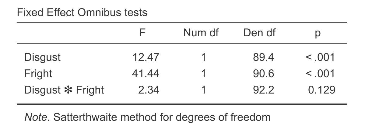
Hopefully this table jumps straight out at you. It looks like an ANOVA table after all. They are the fixed effects, and we can interpret as fixed effects of a classical ANOVA. From this we can see a highly significant effect of Fright and Disgust, but a non-significant interaction.
We can compare these results with what we’d get with a repeated measures ANOVA:
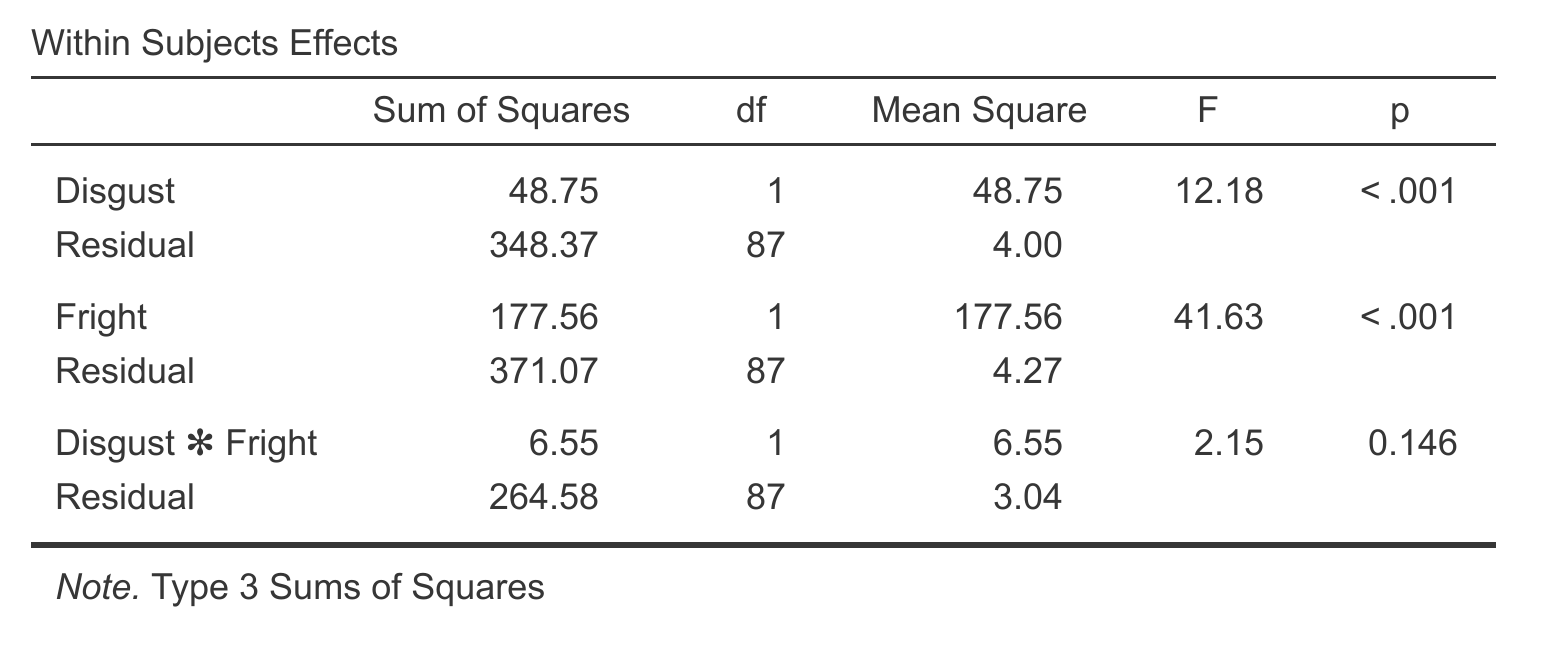
There’s not a huge difference here, but we can see that for the interaction effect the p-value is lower for the linear mixed effects model, which is likely a result of the linear mixed effects model being able to make use of those extra participants that the RM ANOVA was unable to use.
Let’s plot the means for each:
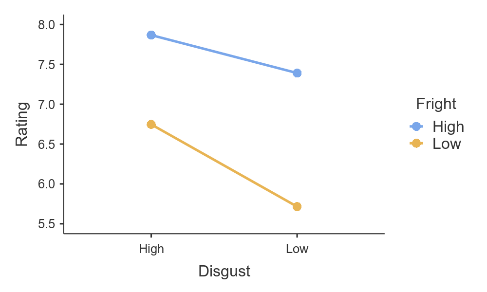
It seems people do want to get rid of highly frightening insects and highly disgusting insects more than others.
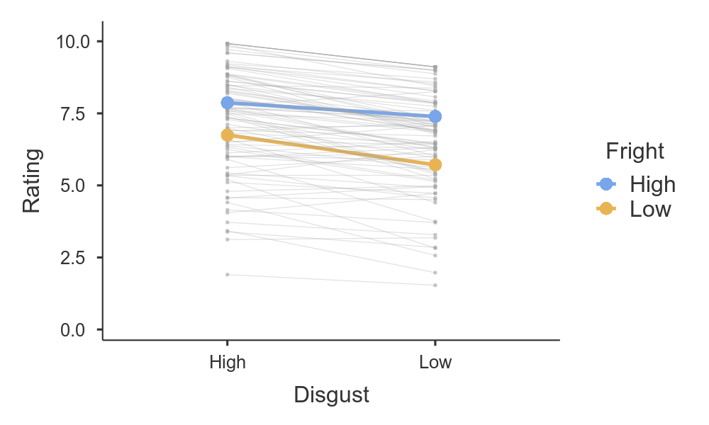
But we can do more than just visualise the marginal means of Fright and Disgust — by checking the random effects box we get a plot of the estimated effect for each subject.
So there we have it, an LME equivalent to Repeated measures ANOVA. Hopefully you can see how approachable these models can be, and that this class of models can become a part of your statistical toolbox. For more examples of Linear mixed models (and General linear models, and Generalised linear models), head on over to the GAMLj docs.
Comments